11.2 Cloud-based geospatial data processing - An advanced example
NDVI computation
var landsat = ee.ImageCollection('LANDSAT/LC08/C02/T1')
    .filterDate('2022-05-01', '2022-10-01')
    .filterBounds(geometry)

print('Number of scenes:', landsat.size())

print("Image collection:", landsat)

// stretch 1 gamma
Map.addLayer(landsat.first(),
             {bands: ["B4", "B3", "B2"]}, "RGB first scene")

var ndvi = landsat.first().normalizedDifference(["B5", "B4"])
print("NDVI first scene", ndvi)
Map.addLayer(ndvi, {min:0, max:1} , "NDVI first scene")

var composite = ee.Algorithms.Landsat.simpleComposite({
  collection: landsat,
  asFloat: true
})

print("Image composite", composite)

Map.addLayer(composite,
             {bands: ["B4", "B3", "B2"], min:0, max: 0.3}, "RGB composite")

var ndvi_composite = composite.normalizedDifference(["B5", "B4"])
print("NDVI composite", ndvi)
Map.addLayer(ndvi_composite, {min:0, max:1} , "NDVI composite")
Tasks
- Play with vizualization parameters
- Change AOI
- Change dates
- Mask clouds
Wildfire analysis
Select AOI and time window based on wildfires reported for 2021 in Greece (Wikipedia).
Task
Import AOI NUTS region (https://geo.fsv.cvut.cz/courses/155isdp/data/11)
Mask clouds
// filter Selntinel-2 L2A based on spatial, temporal and metadata
var s2 = ee.ImageCollection('COPERNICUS/S2_SR')
  .filterBounds(geometry)
  .filterDate('2021-08-01', '2021-10-01')
  .filter(ee.Filter.lt('CLOUDY_PIXEL_PERCENTAGE', 20));

print("Scenes:", s2);

// cloud mask based on QA layer
function mask_clouds(image) {
  // Opaque and cirrus cloud masks cause bits 10 and 11 in QA60
  // to be set, so values less than 1024 are cloud-free
  var mask = ee.Image(0).where(image.select('QA60').gte(1024), 1).not();
  return image.updateMask(mask);
}

// apply on image collection
var s2_masked = s2.map(mask_clouds);

// compare result
Map.addLayer(s2_masked.first(),
            {min: 0, max: 3000, bands: ["B4", "B3" , "B2"]},
            "RGB Image (masked)");
Map.addLayer(s2.first(),
            {min: 0, max: 3000, bands: ["B4", "B3" , "B2"]},
            "RGB Image");
Compute NBR
Normalized Burn Ratio (NBR) is an index designed to highlight burnt areas in large fire zones (link).
// compute normalized burn ratio
function add_NBR(image) {
  return image.addBands(image.normalizedDifference(['B8', 'B12']).rename('NBR'));
};

var s2_nbr = s2_masked.map(add_NBR);

print(s2_nbr)

// NBR before fire appeared
var image0 = s2_nbr.first();
print(ee.Date(image0.get('system:time_start')));
Map.addLayer(image0,
            {min: -1, max: 1, bands: ["NBR"]},
            "NBR Image (before)");

// NBR after fire appeared
var image1 = ee.Image(s2_nbr.toList(1, 1).get(0));
print(ee.Date(image1.get('system:time_start')));
Map.addLayer(image1,
            {min: -1, max: 1, bands: ["NBR"]},
            "NBR Image (after)");
NBR time-series of the burned areas can be displayed by ui.Chart.image.series.
var TSChart = ui.Chart.image.series({
    imageCollection: s2_nbr.select(['NBR']),
    region: geometry,
    reducer: ee.Reducer.mean(),
    scale: 10,
}).setOptions({
    title: 'NBR time-series of the burned areas'
});

print(TSChart);
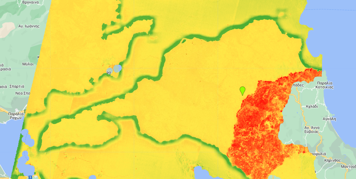
Let's compute burn severity:
var dNBR = ee.Image().expression({
  expression: 'image0.NBR - image1.NBR',
  map: {image0: image0, image1: image1}
}).rename('dNBR');
Map.addLayer(dNBR,
            {min: -1, max: 1, bands: ["dNBR"]},
            "NBR Image (diff)");
Export image: