7.2 Spatio-temporal processing in GRASS GIS
Note
Inspired by Jena GRASS GIS Workshop.
MODIS
The Moderate Resolution Imaging Spectroradiometer MODIS is a 36-channel from visible to thermal-infrared sensor that was launched as part of the Terra satellite payload in December 1999 and Aqua satellite in May 2002. The Terra satellite passes twice a day (at 10:30am and 22:30pm local time), the Aqua satellite also passes twice a day (at 01:30am and 13:30pm local time). (source: GRASS Wiki)
Our area of interest, Germany, is covered by two MODIS tiles (see MODLAND grid):
- h18v03
- h18v04
Data preparation
MODIS data is provided in 3 projections (Sinusoidal, Lambert Azimuthal Equal-Area, and Geographic). For our purpose, data will be reprojected to ETRS89 / LAEA Europe (EPSG:3035).
Create a new GRASS location modis-lst using EPSG code (Select CRS from a list by EPSG or description).
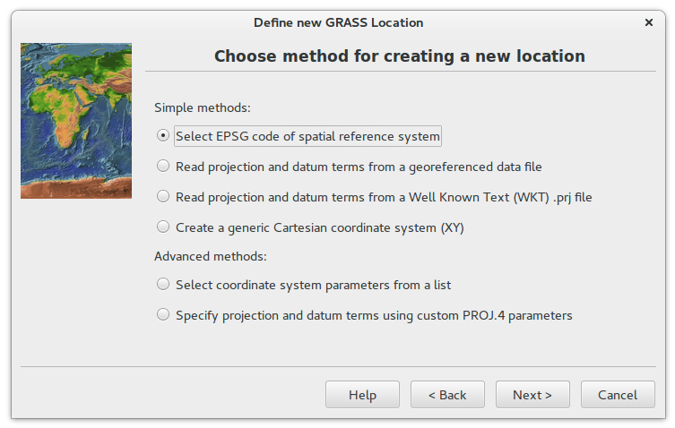 Create a new location based on EPSG code.
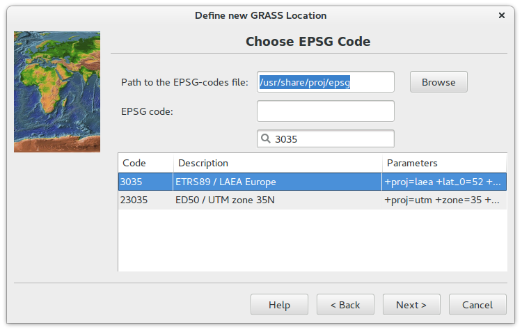 Enter EPSG code.
Enter a new GRASS session (PERMANENT mapset) and install i.modis
addons extension for downloading and importing MODIS data (note that
you have to install also pyMODIS Python
Library). Run two commands below in
Console tab.
GRASS MODIS addon consists of two modules:
Download MODIS data
Note
Pre-downloaded MODIS data (year 2019) is available at https://geo.fsv.cvut.cz/courses/155isdp/data/07/.
Data have been download by i.modis.download tool:
i.modis.download settings=/data/settings.txt folder=/data/de2019 tiles=h18v03,h18v04
     product=lst_aqua_eight_1000,lst_terra_eight_1000 \
     startday=2019-01-01 endday=2019-12-31
Import MODIS data
Input MODIS data can be imported and reprojected into target location
by i.modis.import:
# Terra
i.modis.import -mw files=de2019/listfileMOD11A2.006.txt \
    spectral='( 1 0 0 0 1 0 0 0 0 0 0 0 )' outfile=tlist-mod.txt

# Aqua
i.modis.import -mw files=de2019/listfileMYD11A2.006.txt \
   spectral='( 1 0 0 0 1 0 0 0 0 0 0 0 )' outfile=tlist-myd.txt
Notes
Mosaic is created only if -m flag is given. The parameter outfile requires -w flag.
For spectral values see MOD11A2 product info.
Specify AOI polygon
Administrative border of Germany may be downloaded for example from OSM database (https://overpass-turbo.eu/):
(
relation
["boundary"="administrative"]
["admin_level"="2"]
["name"="Deutschland"]
);
/*added by auto repair*/
(._;>;);
/*end of auto repair*/
out;
Note
Pre-downloaded AOI layer is available at https://geo.fsv.cvut.cz/courses/155isdp/data/07/modis/germany_boundary.gpkg.
The input file contains national border represented by linestring, see figure below (left part). But a mask can be created only from area features (polygons). Input data have to be polygonized. This will be performed by two GRASS operations:
- change line border to boundary by
v.type(in GRASS topological model, an area is composition of boundaries and centroid) - add centroid by
v.centroids
v.type input=germany_boundary output=germany_b from_type=line to_type=boundary
v.centroids input=germany_b output=germany
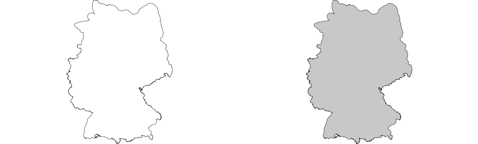 Germany national boundary as linestring on left and as polygon
(area) on right part.
Germany national boundary as linestring on left and as polygon
(area) on right part.
Mask will be created by r.mask. Don't forget that computational
region must be set before creating a mask. Computational region will
be defined by Germany vector map and aligned by the input MODIS data
by g.region.
LST computation
In order to determine Land Surface Temperature (LST) from input data, digital values (DN) must be converted into Celsius or Kelvin scale.
Conversion to Celsium scale can be done by r.mapcalc. It's also
suitable to replace zero values with no-data value (NULL value in
GRASS terminology).
r.mapcalc expression="MOD11A2.A2019001_mosaic_LST_Day_1km_c = \
   if(MOD11A2.A2019001_mosaic_LST_Day_1km != 0, \
   MOD11A2.A2019001_mosaic_LST_Day_1km * 0.02 - 273.15, null())"
Let's check range values of new LST data layer.
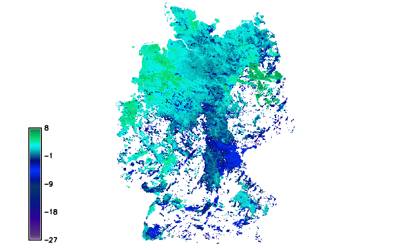 LST reconstruction for Germany in Celsius scale (color table
celsius applied by r.colors tool).
Space-time LST computation
A new space time raster datasets is created by t.create.
In the next step imported MODIS data is registered into space time
dataset by t.register. The command needs to be run twice, once for
Aqua data than for Terra data.
Let's check basic metedata about created dataset by t.info.
...
| Start time:................. 2019-01-01 00:00:00
| End time:................... 2020-01-04 00:00:00
...
| Number of registered maps:.. 184
Note
Check granularity by t.rast.list command. In this case a composed product from the daily 1-kilometer LST product (MOD11A1/MYD11A1) stored on a 1-km Sinusoidal grid as the average values of clear-sky LSTs during an 8-day period is used.
Digital numbers (DN) need to be converted into Celsius scale. Instead
of running r.mapcalc repeatedly there is a specialized temporal
command t.rast.mapcalc which applies map algebra to all the maps
registered in input space time dataset.
Tip
Many temporal data processing modules (t.*) support parallelization (see nproc option).
t.rast.mapcalc input=modis output=modis_c nproc=3 basename=c \
   expression="if(modis != 0, modis * 0.02 - 273.15, null())"
The command will create a new space time raster dataset with raster
maps in Celsius scale. Since new raster maps will be created, the
command requires to define basename. Note that new raster maps will
be produced in the current computation region with mask respected.
id|start|end|mean|min|max|mean_of_abs|stddev|variance|coeff_var|sum|null_cells|cells
c_033@PERMANENT|2019-03-06 00:00:00|2019-03-14 00:00:00|8.38271624724276|-20.35|17.81|...
Color table for all the maps in a space time raster dataset can be set
by t.rast.colors similarly as r.colors does
for a single raster map.
Space-time data aggregation
The temporal framework enables a user to perform data aggregation by
t.rast.aggregate. Based on specified granularity a new temporal
dataset with aggregated data is created.
Statistics can be computed by t.rast.univar.
Example for July and August only.
Space-time data extraction
A new space time dataset only with subset of data can be created by
t.rast.extract. Example for the four seasons below.
t.rast.extract input=modis_c where="start_time > '2019-03-01' and start_time < '2019-06-01'" \
   output=modis_spring

t.rast.extract input=modis_c where="start_time > '2019-06-01' and start_time < '2019-09-01'" \
   output=modis_summer

t.rast.extract input=modis_c where="start_time > '2019-09-01' and start_time < '2019-12-01'" \
   output=modis_autumn

t.rast.extract input=modis_c where="start_time > '2019-12-01' or start_time < '2019-03-01'" \
   output=modis_winter
Another aggregation method is based on t.rast.series. It allows to
aggregate space time raster dataset or part of it by various
methods. The module returns a single raster map as output. In example
below average temperature for each seasons will be computed.
t.rast.series input=modis_spring output=modis_spring_avg method=average
t.rast.series input=modis_summer output=modis_summer_avg method=average
t.rast.series input=modis_autumn output=modis_autumn_avg method=average
t.rast.series input=modis_winter output=modis_winter_avg method=average
Univariate statistics of created raster map with average temperature
values can be calculated by r.univar.
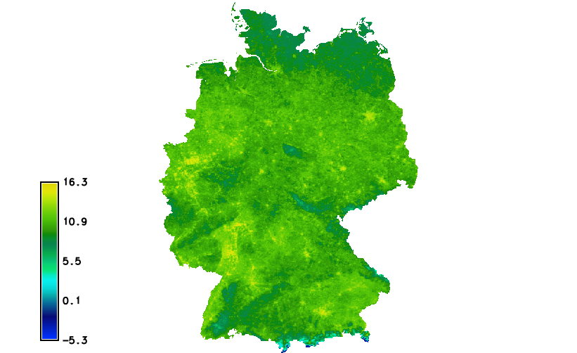 Average temperature for spring 2019.
Space-time data visualization
There are two GRASS tools for temporal data visualization:
g.gui.animation(Temporal -> GUI tools -> Animation tool) andg.gui.tplot(Temporal -> GUI tools -> Temporal plot tool).
Tool g.gui.animation allows creating animations in different
formats, the example below showing the monthly average values.
 Monthly average dataset animation with celsius color table applied.